So you’ve watched all the tutorials. You now understand how a neural network works. You’ve built a cat and dog classifier. You tried your hand at a half-decent character-level RNN. You’re just one pip install tensorflow away from building the terminator, right? Wrong.

A very important part of deep learning is finding the right hyperparameters. These are numbers that the model cannot learn.

In this article, I’ll walk you through some of the most common (and important) hyperparameters that you’ll encounter on your road to the #1 spot on the Kaggle leaderboards. In addition, I’ll also show you some powerful algorithms that can help you choose your hyperparameters wisely.

Hyperparameters in Deep Learning

Hyperparameters can be thought of as the tuning knobs of your model.

A fancy 7.1 Dolby Atmos home theatre system with a subwoofer that produces bass beyond the human ear’s audible range is useless if you set your AV receiver to stereo.

Similarly, an inception_v3 with a trillion parameters won’t even get you past MNIST if your hyperparameters are off.

So now, let’s take a look at the knobs to tune before we get into how to dial in the right settings.

Learning Rate

Arguably the most important hyperparameter, the learning rate, roughly speaking, controls how fast your neural net “learns”.

So why don’t we just amp this up and live life on the fast lane?

Not that simple. Remember, in deep learning, our goal is to minimize a loss function. If the learning rate is too high, our loss will start jumping all over the place and never converge.

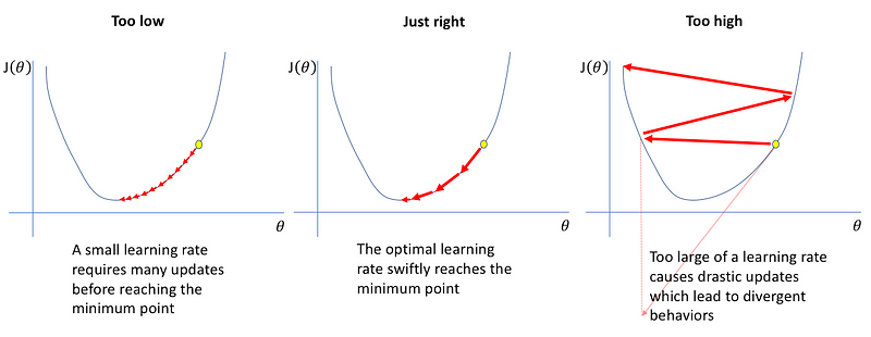
And if the learning rate is too small, the model will take way too long to converge, as illustrated above.

Momentum

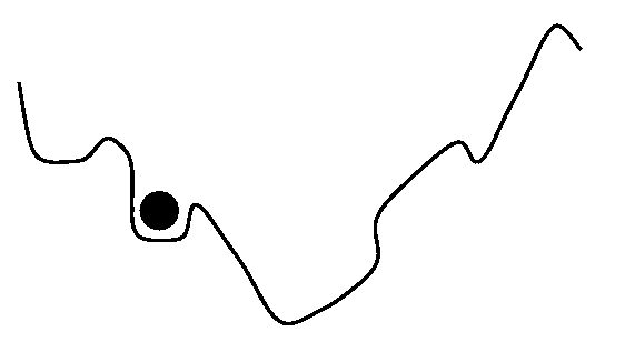
Since this article focuses on hyperparameter optimization, I’m not going to explain the whole concept of momentum. But in short, the momentum constant can be thought of as the mass of a ball that’s rolling down the surface of the loss function.

The heavier the ball, the quicker it falls. But if it’s too heavy, it can get stuck or overshoot the target.

Dropout

If you’re sensing a theme here, I’m now going to direct you to Amar Budhiraja’s article on dropout.

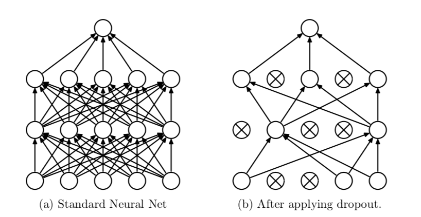
But as a quick refresher, dropout is a regularization technique proposed by Geoff Hinton that randomly sets activations in a neural network to 0 with a probability of (p). This helps prevent neural nets from overfitting (memorizing) the data as opposed to learning it.

(p) is a hyperparameter.

Architecture — Number of Layers, Neurons Per Layer, etc.

Another (fairly recent) idea is to make the architecture of the neural network itself a hyperparameter.

Although we generally don’t make machines figure out the architecture of our models (otherwise AI researchers would lose their jobs), some new techniques like Neural Architecture Search have been implemented this idea with varying degrees of success.

If you’ve heard of AutoML, this is basically how Google does it: make everything a hyperparameter and then throw a billion TPUs at the problem and let it solve itself.

But for the vast majority of us who just want to classify cats and dogs with a budget machine cobbled together after a Black Friday sale, it’s about time we figured out how to make those deep learning models actually work.

Hyperparameter Optimization Algorithms

Grid Search

This is the simplest possible way to get good hyperparameters. It’s literally just brute force.

The Algorithm: Try out a bunch of hyperparameters from a given set of hyperparameters, and see what works best.

Try it in a notebook

The Pros: It’s easy enough for a fifth grader to implement. Can be easily parallelized.

The Cons: As you probably guessed, it’s insanely computationally expensive(as all brute force methods are).

Should I use it: Probably not. Grid search is terribly inefficient. Even if you want to keep it simple, you’re better off using random search.

Random Search

It’s all in the name — random search searches. Randomly.

The Algorithm: Try out a bunch of random hyperparameters from a uniform distribution over some hyperparameter space, and see what works best.

Try it in a notebook

The Pros: Can be easily parallelized. Just as simple as grid search, but a bit better performance, as illustrated below:

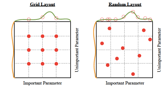
The Cons: While it gives better performance than grid search, it is still just as computationally intensive.

Should I use it: If trivial parallelization and simplicity are of utmost importance, go for it. But if you can spare the time and effort, you’ll be rewarded big time by using Bayesian Optimization.

Bayesian Optimization

Unlike the other methods we’ve seen so far, Bayesian optimization uses knowledge of previous iterations of the algorithm. With grid search and random search, each hyperparameter guess is independent. But with Bayesian methods, each time we select and try out different hyperparameters, the inches toward perfection.

The ideas behind Bayesian hyperparameter tuning are long and detail-rich. So to avoid too many rabbit holes, I’ll give you the gist here. But be sure to read up on Gaussian processes and Bayesian optimization in general, if that’s the sort of thing you’re interested in.

Remember, the reason we’re using these hyperparameter tuning algorithms is that it’s infeasible to actually evaluate multiple hyperparameter choices individually. For example, let’s say we wanted to find a good learning rate manually. This would involve setting a learning rate, training your model, evaluating it, selecting a different learning rate, training you model from scratch again, re-evaluating it, and the cycle continues.

The problem is, “training your model” can take up to days (depending on the complexity of the problem) to finish. So you would only be able to try a few learning rates by the time the paper submission deadline for the conference turns up. And what do you know, you haven’t even started playing with the momentum. Oops.

The Algorithm: Bayesian methods attempt to build a function (more accurately, a probability distribution over possible function) that estimates how good your model might be for a certain choice of hyperparameters. By using this approximate function (called a surrogate function in literature), you don’t have to go through the set, train, evaluate loop too many time, since you can just optimize the hyperparameters to the surrogate function.

As an example, say we want to minimize this function (think of it like a proxy for your model’s loss function):

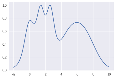
The surrogate function comes from something called a Gaussian process (note: there are other ways to model the surrogate function, but I’ll use a Gaussian process). Like, I mentioned, I won’t be doing any math heavy derivations, but here’s what all that talk about Bayesians and Gaussians boils down to:

$$ mathbb{P} (F_n(X)|X_n) = frac{e^{-frac12 F_n^T Sigma_n^{-1} F_n}}{sqrt{(2pi)^n |Sigma_n|}} $$

Which, admittedly is a mouthful. But let’s try to break it down.

The left-hand side is telling you that a probability distribution is involved (given the presence of the fancy looking ( mathbb{P} ) ). Looking inside the brackets, we can see that it’s a probability distribution of ( F_n(X) ), which is some arbitrary function. Why? Because remember, we’re defining a probability distribution over allpossible functions, not just a particular one. In essence, the left-hand side says that the probability that the true function that maps hyperparameters to the model’s metrics (like validation accuracy, log likelihood, test error rate, etc.) is ( F_n(X) ), given some sample data (X_n) is equal to whatever’s on the right-hand side.

Now that we have the function to optimize, we optimize it.

Here’s what the Gaussian process will look like before we start the optimization process:

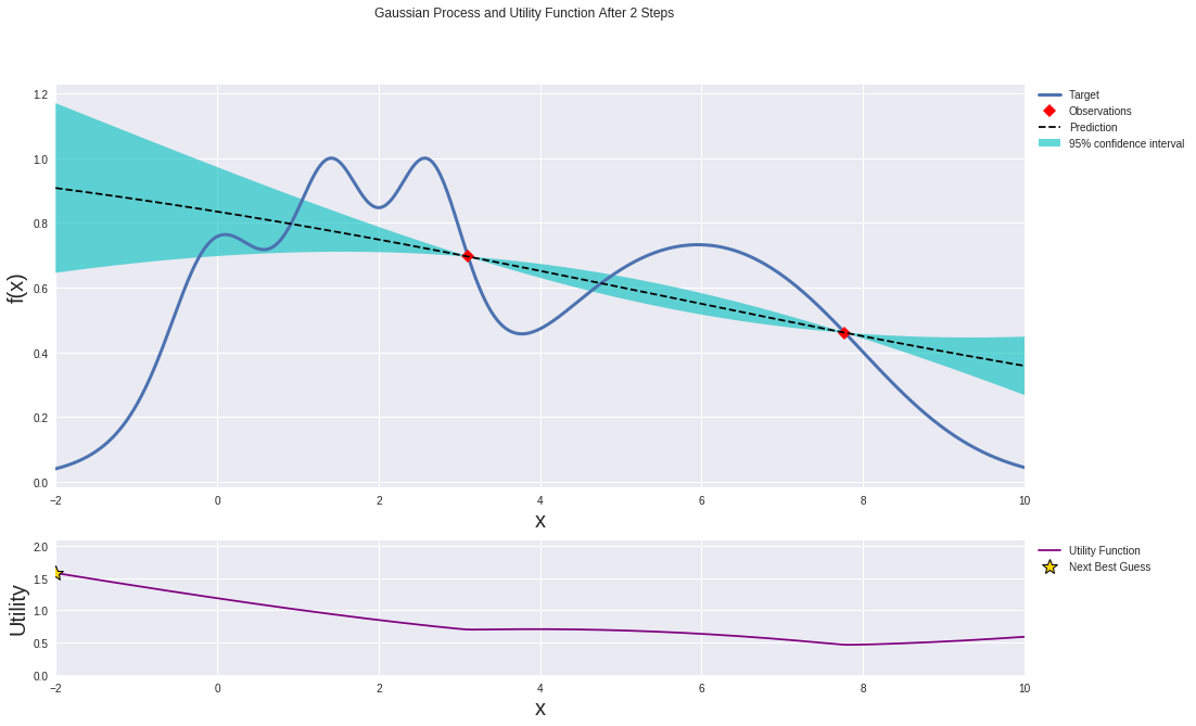
Use your favorite optimizer of choice (the pros like maximizing expected improvement), but somehow, just follow the signs (or gradients) and before you know it, you’ll end up at your local minima.

After a few iterations, the Gaussian process gets better at approximating the target function:

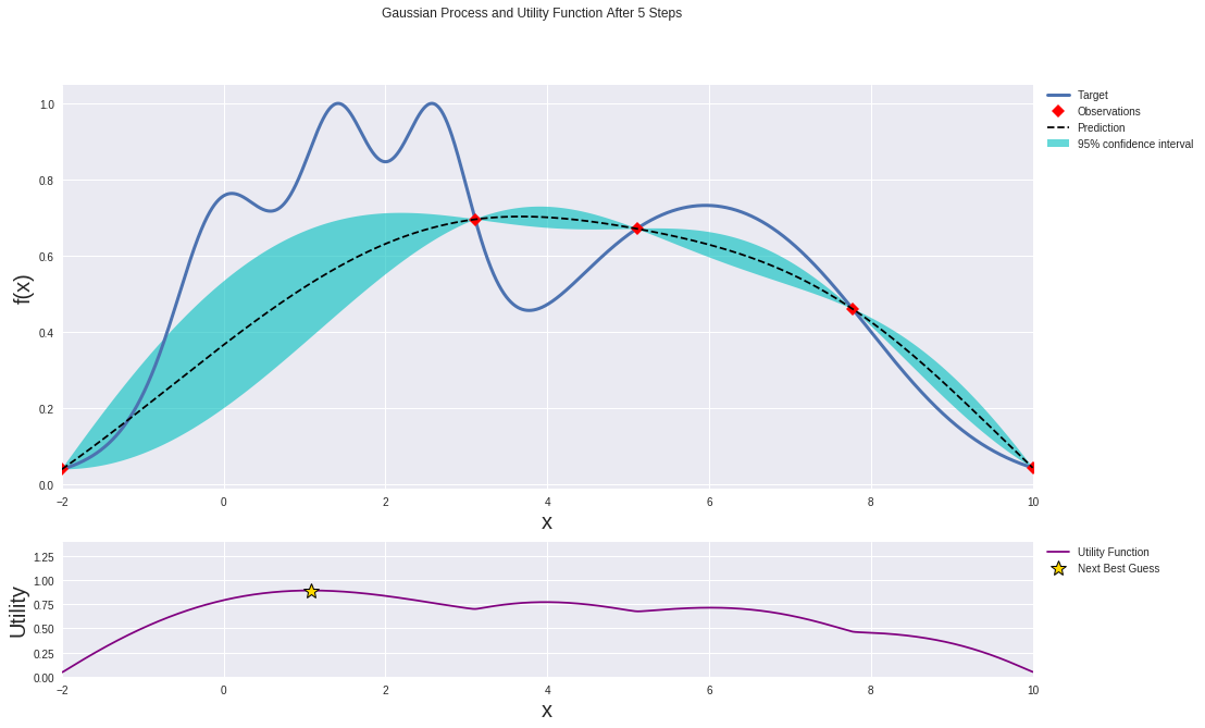
Regardless of the method you used, you have now found the `argmin` of the surrogate function. Ans surprise, surprise, those arguments that minimize the surrogate function are (an estimate of) the optimal hyperparameters! Yay.

The final result should look like this:

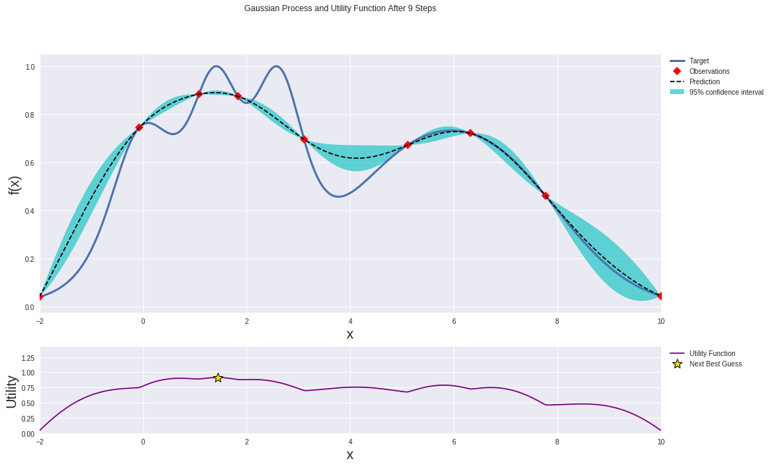
Use these “optimal” hyperparameters to do a training run on your neural net, and you should see some improvement. But you can also use this new information to redo the whole Bayesian optimization process, again, and again, and again. Feel free to run the Bayesian loop however many times you want, but be wary. You are actually computing stuff. Those AWS credits don’t come for free, you know. Or do they…

Try it in a notebook

The Pros: Bayesian optimization gives better results than both grid search and random search.

The Cons: It’s not as easy to parallelize.

Should I Use It: In most cases, yes! The only exceptions would be if

• You’re a deep learning expert and you don’t need the help of a measly approximation algorithm.
• You have access to a vast computational resources and can massively parallelize grid search and random search.
• If you’re an frequentist/anti-Bayesian statistics nerd.

An Alternate Approach To Finding A Good Learning Rate

In all the methods we’ve seen so far, there’s one underlying theme: automate the job of the machine learning engineer. Which is great and all; until your boss gets wind of this and decides to replace you with 4 RTX Titan cards. Huh. Guess you should have stuck to manual search.

But do not despair, there is active research in the field of making researchers do less and simultaneously get paid more. And one of the ideas that has worked extremely well is the learning rate range test, which, to the best of my knowledge, first appeared in a paper by Leslie Smith.

The paper is actually about a method for scheduling (changing) the learning rate over time. The LR (learning rate) range test was a gold nugget that the author just casually dropped on the side.

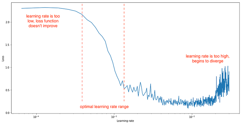
When you’re using a learning rate schedule that varies the learning rate from a minimum to maximum value, such as cyclic learning rates or stochastic gradient descent with warm restarts, the author suggests linearly increasing the learning rate after each iteration from a small to a large value (say, 1e-7 to 1e-1), evaluate the loss at each iteration, and plot the loss (or test error or accuracy) against the learning rate on a log scale. Your plot should look something like this:

Try it in a notebook

As marked on the plot, you’d then use set your learning rate schedule to bounce between the minimum and maximum learning rate, which are found by looking at the plot and trying to eyeball the region with the steepest gradient.

Here’s a sample LR range test plot (DenseNet trained on CIFAR10) from our Colab notebook:

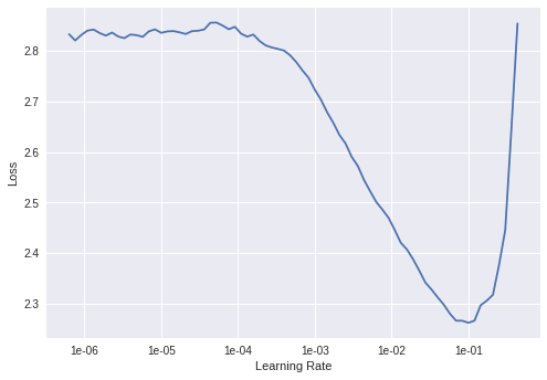
As a rule of thumb, if you’re not doing any fancy learning rate schedule stuff, just set your constant learning rate to an order of magnitude lower than the minimum value on the plot. In this case that would be roughly 1e-2.

The coolest part about this method, other than that it works really well and spares you the time, mental effort, and compute required to find good hyperparameters with other algorithms, is that it costs virtually no extra compute.

While the other algorithms, namely grid search, random search, and Bayesian Optimization, require you to run a whole project tangential to your goal of training a good neural net, the LR range test is just executing a simple, regular training loop, and keeping track of a few variables along the way.

Here’s the type of convergence speed you can expect when using a optimal learning rate (from the example in the notebook):

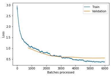
The LR range test has been implemented by the team at fast.ai, and you should definitely take a look at their library to implement the LR range test (they call it the learning rate finder) as well as many other algorithms with ease.

For The More Sophisticated Deep Learning Practitioner

If you’re interested, there’s also a notebook written in pure pytorch that implements the above.  This might give you a better understanding of the behind-the-scenes training process. Check it out here.

Save Yourself The Effort

Of course, all these algorithms, as great as they are, don’t always work in practice. There are many more factors to consider when training neural nets, such as how you’re going to preprocess your data, define your model, and actually get a computer powerful enough to run the darn thing.

Nanonets provides easy to use APIs to train and deploy custom deep learning models. It takes care of all of the heavy lifting, including data augmentation, transfer learning and yes, hyperparameter optimization!

Nanonets makes use of Bayesian search on their vast GPU clusters to find the right set of hyperparameters without the need for you to worry about blowing cash on the latest graphics card and out of bounds for axis 0.

Once it finds the best model, Nanonets serves it on their cloud for you to test the model using their web interface or to integrate it into your program using 2 lines of code.

Say goodbye to less than perfect models.

Conclusion

In this article, we’ve talked about hyperparameters and a few methods of optimizing them. But what does it all mean?

As we try harder and harder to democratize AI technology, automated hyperparameter tuning is probably a step in the right direction. It allows regular folks like you and me to build amazing deep learning applications without a math PhD.

While you could argue that making model hungry for computing power leaves the very best models in the hands of those that can afford said computing power, cloud services like AWS and Nanonets help democratize access to powerful machines, making deep learning far more accessible.

But more fundamentally, what we’re actually doing here using math to solve more math. Which is interesting not only because of how meta that sounds, but also because of how easily it can be misinterpreted.

We certainly have come a long way from the era of punch cards and trace tables to an age where we optimize functions that optimize functions that optimize functions. But we are nowhere close to building machines that can “think” on their own.

And that’s not discouraging, not in the least, because if humanity can do so much with so little, imagine what the future holds, when our visions become something that we can actually see.

And so we sit, on a cushioned mesh chair staring at a blank terminal screen, every keystroke giving us a sudo superpower that can wipe the disk clean.

And so we sit, we sit there all day, because the next big breakthrough might be just one pip install away.

Lazy to code? Don’t want to spend on compute resources? Head over to Nanonets and Start Building a Model now!

You might be interested in our latest posts on: