Last Updated on July 31, 2021

Higher-order derivatives can capture information about a function that first-order derivatives on their own cannot capture. 

First-order derivatives can capture important information, such as the rate of change, but on their own they cannot distinguish between local minima or maxima, where the rate of change is zero for both. Several optimization algorithms address this limitation by exploiting the use of higher-order derivatives, such as in Newton’s method where the second-order derivatives are used to reach the local minimum of an optimization function. 

In this tutorial, you will discover how to compute higher-order univariate and multivariate derivatives. 

After completing this tutorial, you will know:

• How to compute the higher-order derivatives of univariate functions. 
• How to compute the higher-order derivatives of multivariate functions.
• How the second-order derivatives can be exploited in machine learning by second-order optimization algorithms.

Let’s get started. 

Higher-Order Derivatives
Photo by Jairph, some rights reserved.

Tutorial Overview

This tutorial is divided into three parts; they are:

• Higher-Order Derivatives of Univariate Functions
• Higher-Order Derivatives of Multivariate Functions
• Application in Machine Learning

Higher-Order Derivatives of Univariate Functions

In addition to first-order derivatives, which we have seen can provide us with important information about a function, such as its instantaneous rate of change, higher-order derivatives can also be equally useful. For example, the second derivative can measure the acceleration of a moving object, or it can help an optimization algorithm distinguish between a local maximum and a local minimum. 

Computing higher-order (second, third or higher) derivatives of univariate functions is not that difficult.

The second derivative of a function is just the derivative of its first derivative. The third derivative is the derivative of the second derivative, the fourth derivative is the derivative of the third, and so on.

– Page 147, Calculus for Dummies, 2016.

Hence, computing higher-order derivatives simply involves differentiating the function repeatedly. In order to do so, we can simply apply our knowledge of the power rule. Let’s consider the function, f(x) = x³ + 2x² – 4x + 1, as an example. Then:

First derivative: f’(x) = 3x² + 4x – 4

Second derivative: f’’(x) = 6x + 4

Third derivative: f’’’(x) = 6

Fourth derivative: f ⁽⁴⁾(x) = 0

Fifth derivative: f ⁽⁵⁾(x) = 0 etc.

What we have done here is that we have first applied the power rule to f(x) to obtain its first derivative, f’(x), then applied the power rule to the first derivative in order to obtain the second, and so on. The derivative will, eventually, go to zero as differentiation is applied repeatedly. 

The application of the product and quotient rules also remains valid in obtaining higher-order derivatives, but their computation can become messier and messier as the order increases. The general Leibniz rule simplifies the task in this aspect, by generalising the product rule to:

Here, the term, n! / k!(n – k)!, is the binomial coefficient from the binomial theorem, while f ^(k) and  g^(k) denote the k^th derivative of the functions, f and g, respectively. 

Therefore, finding the first and second derivatives (and, hence, substituting for n = 1 and n = 2, respectively), by the general Leibniz rule, gives us:

(fg)⁽¹⁾ = (fg)’ = f ⁽¹⁾ g + f g⁽¹⁾

(fg)⁽²⁾ = (fg)’’ = f ⁽²⁾ g + 2f ⁽¹⁾ g⁽¹⁾ + f g⁽²⁾

Notice the familiar first derivative as defined by the product rule. The Leibniz rule can also be used to find higher-order derivatives of rational functions, since the quotient can be effectively expressed into a product of the form, f g^-1. 

Higher-Order Derivatives of Multivariate Functions

The definition of higher-order partial derivatives of multivariate functions is analogous to the univariate case: the n^th order partial derivative for n > 1, is computed as the partial derivative of the (n – 1)^th order partial derivative. For example, taking the second partial derivative of a function with two variables results in four, second partial derivatives: two own partial derivatives, f_xx and f_yy, and two cross partial derivatives, f_xy and f_yx. 

To take a “derivative,” we must take a partial derivative with respect to x or y, and there are four ways to do it: x then x, x then y, y then x, y then y.

– Page 371, Single and Multivariable Calculus, 2020.

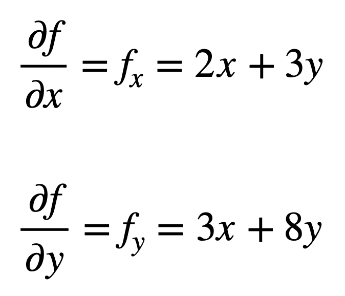
Let’s consider the multivariate function, f(x, y) = x² + 3xy + 4y², for which we would like to find the second partial derivatives. The process starts with finding its first-order partial derivatives, first:

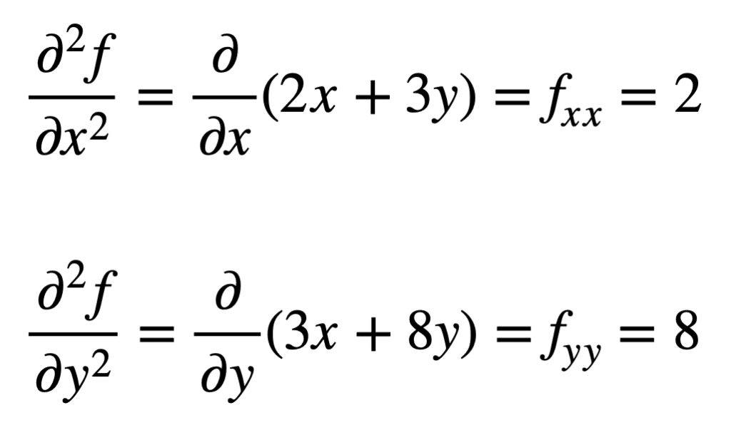
The four, second-order partial derivatives are then found by repeating the process of finding the partial derivatives, of the partial derivatives. The own partial derivatives are the most straightforward to find, since we simply repeat the partial differentiation process, with respect to either x or y, a second time:

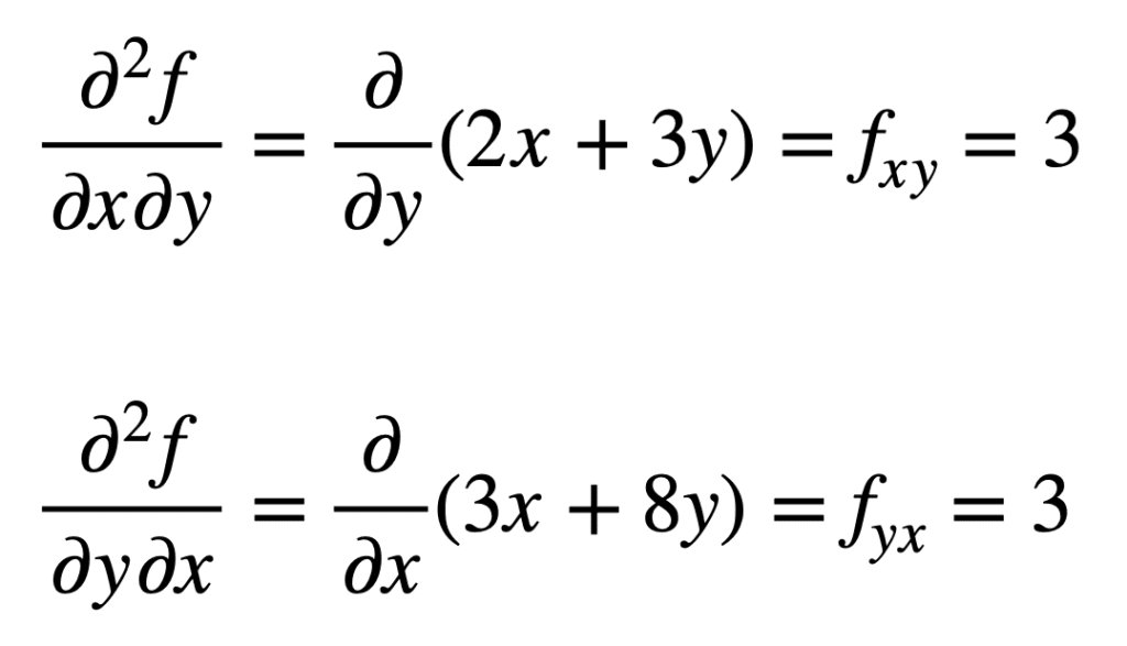
The cross partial derivative of the previously found f_x (that is, the partial derivative with respect to x) is found by taking the partial derivative of the result with respect to y, giving us f_xy. Similarly, taking the partial derivative of f_y with respect to x, gives us f_yx: 

It is not by accident that the cross partial derivatives give the same result. This is defined by Clairaut’s theorem, which states that as long as the cross partial derivatives are continuous, then they are equal. 

Application in Machine Learning

In machine learning, it is the second-order derivative that is mostly used. We had previously mentioned that the second derivative can provide us with information that the first derivative on its own cannot capture. Specifically, it can tell us whether a critical point is a local minimum or maximum (based on whether the second derivative is greater or smaller than zero, respectively), for which the first derivative would, otherwise, be zero in both cases. 

There are several second-order optimization algorithms that leverage this information, one of which is Newton’s method.

Second-order information, on the other hand, allows us to make a quadratic approximation of the objective function and approximate the right step size to reach a local minimum …

– Page 87, Algorithms for Optimization, 2019.

In the univariate case, Newton’s method uses a second-order Taylor series expansion to perform the quadratic approximation around some point on the objective function. The update rule for Newton’s method, which is obtained by setting the derivative to zero and solving for the root, involves a division operation by the second derivative. If Newton’s method is extended to multivariate optimization, the derivative is replaced by the gradient, while the reciprocal of the second derivative is replaced with the inverse of the Hessian matrix. 

We shall be covering the Hessian and Taylor Series approximations, which leverage the use of higher-order derivatives, in separate tutorials. 

Further Reading

This section provides more resources on the topic if you are looking to go deeper.

Books

Summary

In this tutorial, you discovered how to compute higher-order univariate and multivariate derivatives. 

Specifically, you learned:

• How to compute the higher-order derivatives of univariate functions. 
• How to compute the higher-order derivatives of multivariate functions.
• How the second-order derivatives can be exploited in machine learning by second-order optimization algorithms. 

Do you have any questions?
Ask your questions in the comments below and I will do my best to answer.